Spatial visualization [visualize]

Setup

We’ll start by loading the tidyverse, sf, and read in a couple of sample datasets.

library(tidyverse)
library(sf)

nc <- read_sf(system.file("shape/nc.shp", package = "sf"))
states <- st_as_sf(maps::map("state", plot = FALSE, fill = TRUE))

`geom_sf()`

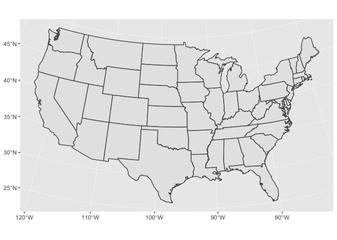
The easiest way to get started is to supply an sf object to geom_sf():

ggplot() +
  geom_sf(data = nc)

Notice that ggplot2 takes care of setting the aspect ratio correctly.

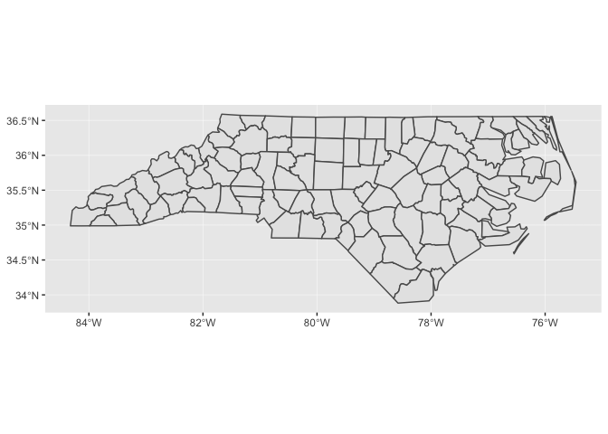
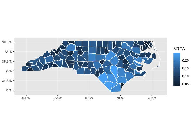
You can supply other aesthetics: for polygons, fill is most useful:

ggplot() +
  geom_sf(aes(fill = AREA), data = nc, color = "white")

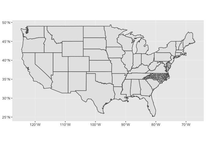
When you include multiple layers, ggplot2 will take care of ensuring that they all have a common coordinate reference system (CRS) so that it makes sense to overlay them.

ggplot() +
  geom_sf(data = states) + 
  geom_sf(data = nc)

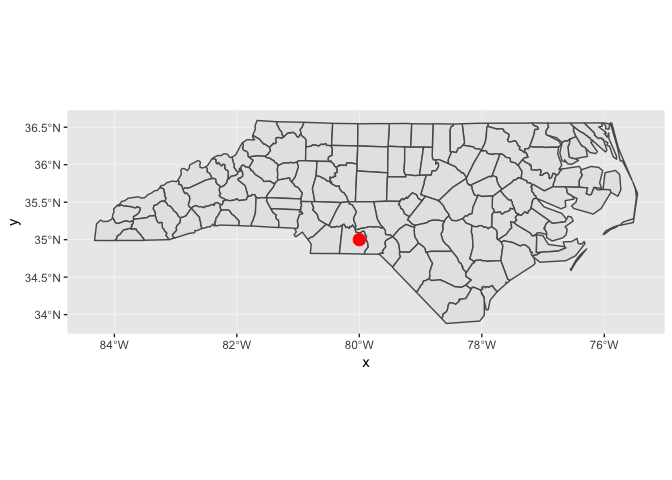
You can combine geom_sf() with other geoms. In this case, x and y positions are assumed be in the same CRS as the sf object (typically these will be longitude and latitude).

ggplot() +
  geom_sf(data = nc) +
  annotate(geom = "point", x = -80, y = 35, color = "red", size = 4)

`coord_sf()`

You’ll need to use coord_sf() for two reasons:

You want to zoom into a specified region of the plot by using xlim and ylim

ggplot() +
  geom_sf(data = nc) +
  annotate(geom = "point", x = -80, y = 35, color = "red", size = 4) + 
  coord_sf(xlim = c(-81, -79), ylim = c(34, 36))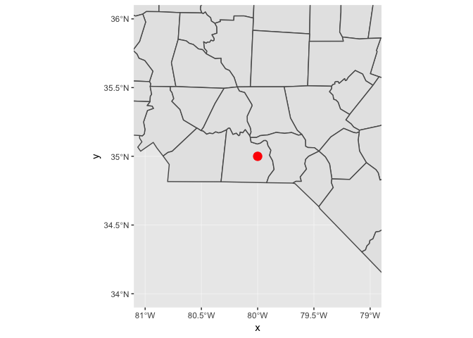

You want to override to use a specific projection. If you don’t specify the crs argument, it just uses the one provided in the first layer. The following example uses an Albers Equal Area projection and the NAD83 datum, with an EPSG code of 102003.
```
ggplot() +
  geom_sf(data = states) +
  coord_sf(crs = st_crs(102003))
```